True Position Process Capability - Other Methods

Introduction

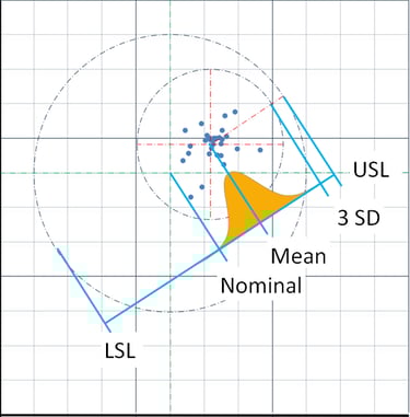
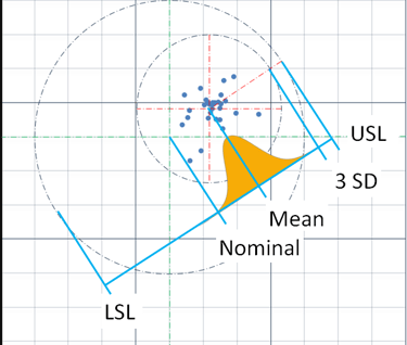
This post is an addendum to an article posted on LinkedIn. That article was shortened to keep it focused on the main objective of describing a better method to determine process capability for circular true position tolerances. Very briefly, you need to find the center of the data points as if plotted on a 2D grid and use the distance from each point to the center point to calculate the standard deviation. The shortcomings of the method of simply finding the process capability of the component dimensions (x, y coordinates) were provided. Here, several other techniques will be given and critiqued.

Alternative method 1

There is a very simple method that provides good results but with some limitations. I discovered this method on an Elsmar Cove forum and it is based on the x, y coordinates method. Instead finding process capability for the x, y coordinates based on a ± tolerance of half of the true position tolerance, take that halved value and further divide by √2, or 1.414. This may look familiar as the circle that contains the points of a .010” x .010” square is .1414”. So, for a true position of Ø.020”, the tolerance to use would be .010”/1.414 or .00707”. The problem with this method is that you get two process capability results instead of just one and they are likely to be different. A small Monte Carlo analysis suggests using the lower value is a pretty good representation. My recommendation would be to use the method detailed in my LindedIn article for a final determination of process capability but use the simplified method for an initial evaluation of the data until you are able to fully analyze it.

Alternative method 2.

Davis R. Bothe addresses this same issue in his 2006 paper in Quality Engineering, Accessing Capability for Hole Location. His method differs in both calculating the radius and standard deviation. In his paper he calculates both short-term capability, Cpk, and long-term capability, Ppk values by using significantly different formulas for the same data. A little on short-term and long-term capability, a topic mostly ignored in the first article. Cpk is an evaluation of the potential for a process and properly uses sup-groups to calculate an estimated standard deviation. Ppk is an evaluation of the performance of a particular lot and uses the standard deviation of the lot in question. Bothe’s method does not use sub-groups to calculate Cpk but it is possible he avoiding doing so to simplify the paper. That said, both of his standard deviation calculations have shortcomings.

To calculate short term sigma, Bothe uses a moving range, MR, chart. The chart records the true position radius. What he then calculates is the absolute change in value from one data point to another. Bothe uses the average of the change, calling it MRbar, to calculate sigma. He defines σ short term as MRbar/1.128. A significant flaw can easily be shown in this application. The standard deviation for a set of data is independent of the order in which the data is gathered. MRbar is dependent on the order of the data. Intuitively this seemed true and a little playing around with Excel confirmed it. The method in my LindedIn article does not have that deficiency; the data can be in any order and provide the same result.

Bothe uses a very different formula to calculate the long-term sigma. His first steps are correct; he calculates the center of the data and then the distance of each data point to the center of the data. His formula for standard deviation includes a summation of (ri – r̅ )^2, where ri is radius of each individual point to the process center and r̅ is the mean of each of those radial values. This is where his mistake is. For standard deviation, it is the distance from each data point to the center of the data that is squared. Bothe has that value in ri. There is no need to subtract from it r̅ , a mean of those radius values. The end result is to make the standard deviation too small, suggesting a more capable process than it really is. This can be seen (sorry, no image) where he calculates Pp to be 4.03 for his sample set of data, meaning there are 12 standard deviations from the center to the limit. Visually, the data points in the graph appear to be more spread out than that Pp would indicate.

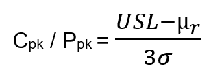
An additional error Bothe makes is in the use of mean radius. His general formula for process capability is:

where µr is the mean of measured true position radius relative to the process center, mean radius. The numerator of the equation expresses the distance from the center of the data set to the specification limit. As explained in the article, the mean radius does not indicate the center of the data set. So, what Bothe enters into the equation does not include the center of the data set and therefore cannot find the distance to the specification limit. In fact, in a case where the center of the data was very close nominal, this equation would miss that fact because it is using mean radius, which will suggest that it is not at nominal.

How the Firearm Industry Does It.

This summary is based on a much more detailed explanation on the Precision Rifle Blog, which in turn quotes other sources, so beware of going into a rabbit hole. The firearms industry, referring to both guns and ammunition, does not use either process capability or standard deviations to evaluate accuracy. Two other methods are used, extreme spread and mean radius, but the preferred method seems to be mean radius. Note this is a different mean radius than used above. To find it for any given pattern of holes in a target, first find the center of the pattern. With that, measure the distance of each hole to the center. Finally, find the average of each of those distances and you have calculated the mean radius. According to the referenced article, there is not agreement that the distribution is normally distributed so they do not go to the next step and calculate a standard deviation. However, they do take the step of using mean radius to predict a radius in which 95% of shots are expected to land. Not a lot of detail is provided in the article but it says for a 10 shot pattern, multiply the mean radius by 2.1 to get the radius where you are confident 95% of the shots will occur, R95. Logically, that multiplication factor should vary by sample size. In this example, knowing that ±2 σ from the mean comprises 95.4% of the data, they are saying that the mean radius and standard deviation, were it calculated, are very close. Recall mean radius used here is of the bullet holes relative to the center of the pattern of holes. Earlier, it referred to the average of the radial distance from the data points to the nominal center. Bothe does not use the term "mean radius" but uses both senses of it in different locations. Nevertheless, the concerns discussed earlier with using mean radius are much less in the way the firearm industry uses it.

So far, we have just considered the spread of the data, or precision, without considering how close it is to the target, or accuracy. In my brief research I have found that called windage and elevation or horizontal and vertical offset. Exactly how that is accounted for is beyond the scope here but I do know that telescopic scopes have adjustments for wind and elevation. I would assume that before using a scope, the gun owner would do some testing of the gun itself to see how accurate it is and either correct errors or account for them in using the scope. Finally, I find it a little surprising that standard deviation is not part of the ammunition and firearm evaluation considering the research and development of all things military throughout time. If anyone can correct me in this area, I would be happy to learn.